Measures of Variation is an important topic in Lean Six Sigma Green Belt certification. What is process variation in Lean Six Sigma? A measure of variation (or dispersion) defines the spread or scattering of the set of obtained data around the central value. The measure of variation in Lean Six Sigma is commonly measured with the following descriptive statistics:

• Range: The range is equal to the largest value minus the smallest value of the data set.
• Interquartile range: The range of the middle half of a distribution
• Standard Deviation: Standard deviation is a measure of how much data values vary away from the mean. The larger the standard deviation means greater the amount of variation.

Measure of variation is an important measurement method that we use in Lean Six Sigma projects. Lean Six Sigma is a new quality initiative revolutionizing process improvement in various industries. This article will cover all the tips and tricks which will help you successfully understand the measures of variation for your process and clear the Lean six sigma certification exam.

Lean Six Sigma stands out for its distinctly process-focused methodology. Rather than merely targeting end results, Six Sigma dives deep into the processes, identifying bottlenecks, eliminating inefficiencies, and ensuring that each step is optimized for maximum value. This process-centric approach allows organizations to not only achieve but also sustain unparalleled levels of quality, making Six Sigma an indispensable tool for those committed to operational excellence.

What is the purpose of measures of variation?

There are many benefits of reducing variation in a process. The measure of variation is significant for some of the following purposes

• Measure of variation determines the reliability of an average by pointing out how far an average is representative of the entire data.
• Another purpose of measuring variability is to determine the nature cause variation to control the variation itself.
• Measures of variation enable comparisons of two or more distributions regarding their variability.
• Measuring variation is of great importance to advanced statistical analysis. For example, sampling or statistical inference is essentially a problem in measuring variability.

Lean Six Sigma is dedicated to reducing variation in processes. Whether it’s common cause variation, which stems from everyday system fluctuations, or special cause variation, which arises from unforeseen or exceptional circumstances, Lean Six Sigma provides tools and methodologies to address both. By reducing these variations, Six Sigma ensures consistent output and product quality. As variation amplifies within a process, so does the risk of defects and inefficiencies.

Measure of Variations in Statistics

Measures of variation in statistics are ways to define the dispersion of your data set. In other words, it shows how far away data points are from each other. Statisticians use measures of variation to review their data set. You can derive many conclusions by using measures of variation, such as high and low variability. High variability can mean that the data is inconsistent. Low variability means data is consistent. You can use measures of variation to measure and analyze trends in your data, which can be applicable to many careers that use statistics. Given below are proven and tested tips by industry experts

There are many ways to describe the measure of variation or spread including-

• Range and Standard Deviation and Interquartile range (IQR)

How to determine the Range?

Range shows the mathematical distance between the lowest and highest values in the data set.

Range measures the variability of the data set.

A wide range indicates greater variability in the data, or perhaps a single outlier far from the rest of the data. Outliers may skew, or shift, the mean value enough to impact data analysis.

For example, the range of 30, 33, 31, 34, 35, 32 and 46

The lowest value is 30 and the highest value is 46.

To calculate the range, subtract the lowest value from the highest value (46−30=16).

The range equals 16.

In the sample set, the high data value of 46 exceeds the previous value, 35, by 11. This value seems extreme, given the other values in the set. The value of 46 might be an outlier data point.

The range is very easy to compute, and it gives us some idea about the variability of the data. However, the range is a crude measure of variation, since it uses only two extreme values.

The concept of range is extensively used in statistical quality control.

Range is helpful in studying the variations in the prices of shares and debentures and other commodities that are very sensitive to price changes from one period to another. For meteorological departments, the range is a good indicator for the weather forecast.

How to determine the Standard Deviation?

Standard deviation measures the variability of the data set. Like range, a smaller standard deviation indicates less variability.

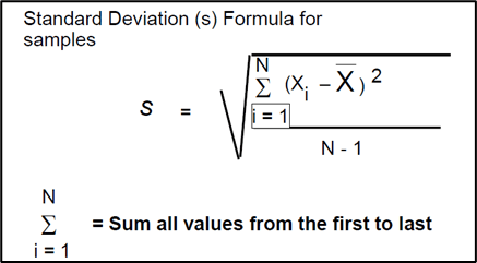
Finding standard deviation for samples requires summing the squared difference between each data point and the mean [∑(​x​ − ​µ​)2], adding all the squares, dividing that sum by one less than the number of values (​N​ − 1), and finally calculating the square root of the dividend. In one formula, this is:

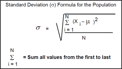
Finding standard deviation for a population requires summing the squared difference between each data point and the mean [∑(​x​ − ​µ​)2], adding all the squares, and dividing that sum by the total population of values (​N​), and finally calculating the square root of the dividend. In one formula, this is:

For example, the sample standard deviation is the square root from the variance and in this case for the five values: 14, 36, 45, 50, 85 is to be calculated as:

N=5 and the mean for x= 46

Xi	Xi-X	(Xi-X)2
14	-32	1024
36	-10	100
45	-1	1
50	4	16
85	39	1521
∑Xi= 230		∑(Xi-X)2=   2662

Substitute the results in the samples standard deviation formula

The standard deviation for the above example is 25.81

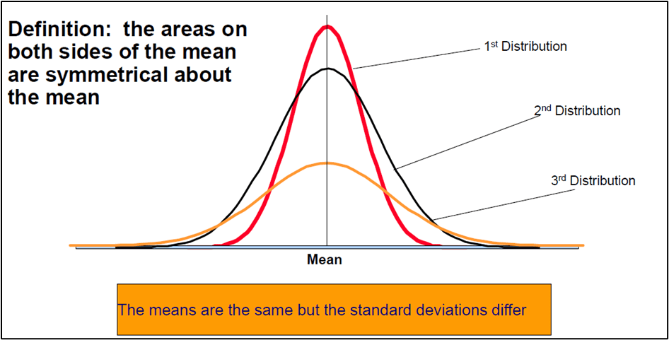
The mean (M) ratings are the same for each group – it’s the value on the x-axis when the curve is at its peak. However, their standard deviations (SD) differ from each other.

The standard deviation reflects the dispersion of the distribution. The curve with the lowest standard deviation has a high peak and a small spread, while the curve with the highest standard deviation is flatter and more widespread.

How to determine the Interquartile range?

Inter Quartile Range (IQR) represents where the middle (50%) of values lie in each range of data. Let’s simplify it further.

Arrange the data in ascending or descending order.

For example, if the data is 3,5,6,7,7,7,2,9,10,12,13

Arrange it in descending order 13,12,10,9,7,7,7,6,5,3,2

Find the middle value or median of the lower and upper half of the data set.

Here the median (mid-point) is 7

Then find the first quartile, Divide below 50% data set into two quartiles. The first quartile is the value under 25% of the data points found when data points.

Here the first quartile is 5

Then find the 3^rd quartile. Divide the above 50% data set into two quartiles. The upper quartile or 3^rd quartile is the value under which 75% of the data points.

Here the third quartile is 10

The formula for finding the interquartile range takes the third quartile value, and subtracts the first quartile value.  IQR = Q3 – Q1

Here the interquartile is IQR=10-5=5

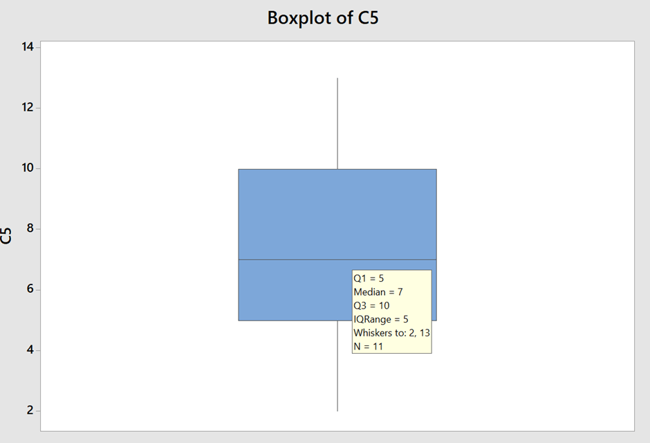
Spacing between each part of the box indicates the degree of dispersion or variation

When can use a box plot?

Spacing between each part of the box indicates the degree of dispersion or variation

When can use a box plot?

• When you have huge amounts of data
• When difficult to analyse the statistical part of the numbers
• Box plot enables a visual summary of the data

Interquartile range= Third quartile(Q3)- First quartile(Q1)

These formulas are used to calculate the process variations

Please answer simple questions given below then compare your answers with answer key:

Measure of variations – Example exercise 1

The range for the following numbers (6, 3, 2, 5, 1, 8,7) is ______

Measure of variations – Example exercise 2

The median for the following numbers (6, 3, 2, 5, 1, 8,7) is _______

Measure of variations – Example exercise 3

A common measure of variation is _______

Answers for skills-building exercises

The answer for the first sample exercise is: 6

The answer for the second sample exercise is: 5

The answer for the third sample exercise is: Range, standard deviation and IQR

Conclusion

Measure of variation can be measured by finding the range, standard deviation, and IQR. The range and the interquartile range use only two values in their calculation. But the IQR is less impacted by outliers: Standard deviation alone serves as a pointer for where to investigate within the process for problems or solutions. To reduce variation in process improvement, standard deviation becomes a significant concept in both analysis and statistical process control and frequently serves as the starting point for further statistical six sigma analysis. Standard deviation is a good measure of variability for normal distributions or distributions that aren’t terribly skewed. Paired with mean this is a good way to describe the data.

Also Read: Lean Six Sigma Green Belt Certification Measure Of Location